0

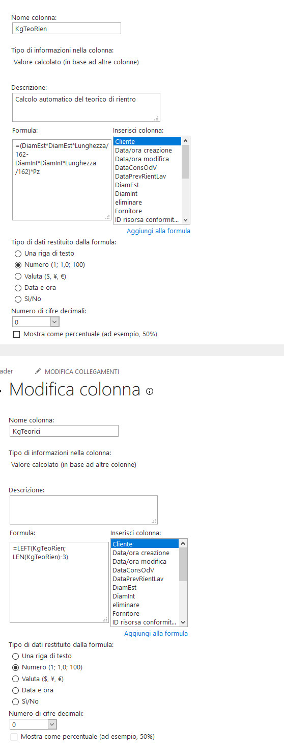
I have a calculated field which is filled in automatically thanks to a simple formula:

=(X*X*Z/162-Y*Y*Z/162)*X

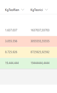
This generate a number like: 1.637.037 I have a problem on adding RIGHT function to remove first 4 char from right to left and leave the number like 1.637 or like 1.637,03 by adding the comma.

Can anyone help me?

Thanks

Update

enter image description here

enter image description here

2
  • Is your column value always has the format like: x.xxx.xxx? 1 digit then 3 digits and 3 digits?? Commented Jan 10, 2020 at 11:14
  • Yes, is a calculated column. Example: =(150,00*150,00*6000,00/162-20,00*20,00*6000,00/162)*2 generate 1.637.037
    – MarkR
    Commented Jan 10, 2020 at 12:05

2 Answers 2

0

Assuming your column name is Column of Type "Single Line of Text" and always has the format like x.xxx.xxx,

Try using below formula:

=LEFT([Column],INT(FIND(".",[Column],3)-1))

Note:

  1. Sometimes comma(,) does not work in calculated column formula (I am not sure but it is based on something language or regional settings on your site). So in that case use semicolon(;) instead of comma(,).
  2. Change the The data type returned from this formula is of your calculated column to Single line of text from column settings.
6
  • In italy Sharepoint convert comma to semicolon automatically. Anyway your formula doesn't work it show me a #VALUE! error on the Sharepoint table.
    – MarkR
    Commented Jan 10, 2020 at 12:44
  • You need to convert your previous calculated column (column in attached image to question) to be of type single line of text instead of number. Commented Jan 10, 2020 at 13:00
  • I done this but it give me the same #VALUE! error.
    – MarkR
    Commented Jan 10, 2020 at 13:13
  • Change the data type for both calculated column (previous and new). Are there any blank values in your previous column for some list items? Commented Jan 10, 2020 at 13:21
  • I can still see that "Number" selected for "The data type returned from this formula is" option (this option is below formula in calculated column settings). Commented Jan 10, 2020 at 13:26
0

May be you need LEFT function?

RIGHT will extract number of characters from the right side.

To remove last 4 characters from right - try to use formula:

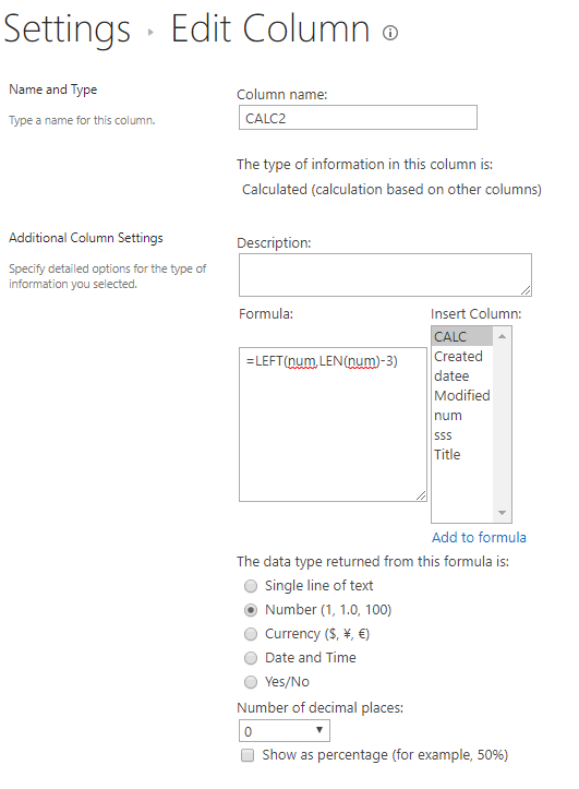
=LEFT([column],LEN([column])-3)

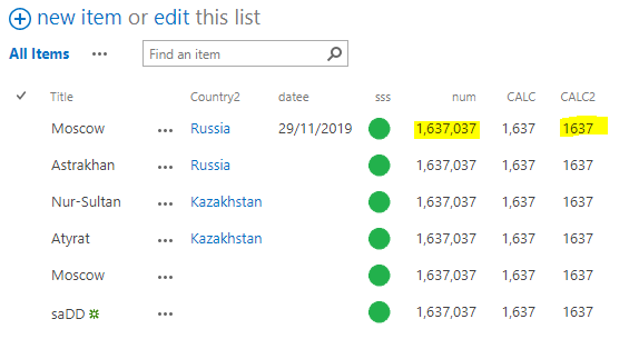
enter image description here enter image description here

11
  • No, in my example I need to remove 4 char from right. 1.637.037 to 1.637 (or 1.637,00)
    – MarkR
    Commented Jan 10, 2020 at 12:22
  • @MarkR you need to use LEFT function to leave left part and exclude right part.
    – Raf
    Commented Jan 10, 2020 at 12:26
  • @MarkR I've updated my answer.
    – Raf
    Commented Jan 10, 2020 at 12:43
  • It doesn't work. It convert it like this: 1.637.37 to 1637037,03703
    – MarkR
    Commented Jan 10, 2020 at 12:58
  • @MarkR look on my screens. As you can see It does not convert to 1637037,03703. It removes last 4 characters from right.
    – Raf
    Commented Jan 10, 2020 at 13:01

Your Answer

By clicking “Post Your Answer”, you agree to our terms of service and acknowledge you have read our privacy policy.

Not the answer you're looking for? Browse other questions tagged or ask your own question.